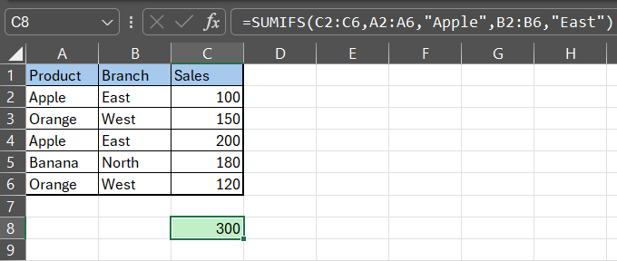
Understanding Multiple Conditional Sum:
Multiple conditional sum in Excel involves calculating the sum of values in a range based on multiple criteria or conditions. Instead of restricting your calculations to a single criterion, you can specify multiple conditions that must be met for a value to be included in the sum. This allows for more targeted and nuanced analysis of your data, enabling you to extract valuable insights and draw meaningful conclusions.
Multiple Conditional Sum:
Excel provides several functions and techniques for performing multiple conditional sum, each offering its own advantages and use cases. Let’s explore some of the most common methods:
SUMIFS Function:
The SUMIFS function is specifically designed for multiple conditional sum. It allows you to specify pairs of range and criteria arguments, with each pair representing a separate condition that must be met.
The relationship between criteria in the SUMIFS function is an “AND” relationship. This means that all specified criteria must be met simultaneously for a value to be included in the sum.
For example, if you have two criteria:
- Salesperson must be “John”
- Sales amount must be greater than 1000
The SUMIFS function would only include sales amounts where both conditions are true: the salesperson is “John” and the sales amount is greater than 1000.
If you want to include values that meet any of the specified criteria (i.e., an “OR” relationship), you would need to use separate SUMIFS functions or alternative approaches such as using helper columns or array formulas.
=SUMIFS(sum_range, criteria_range1, criteria1, [criteria_range2, criteria2], ...)
sum_range: This is the range of cells that you want to sum if the corresponding cells meet all of the specified criteria.criteria_range1, criteria_range2, ...: These are the ranges of cells that contain the values you want to evaluate against the specified criteria. You can specify multiple pairs of criteria_range and criteria.criteria1, criteria2, ...: These are the criteria that must be met for the corresponding cells in the criteria_range. You can specify multiple criteria.
Here’s a breakdown of how to interpret each part of the syntax:
sum_range: This is the range of cells that you want to sum. For example, if you want to sum sales figures, you would specify the range of cells containing the sales data.criteria_range1, criteria_range2, ...: These are the ranges of cells that contain the values you want to evaluate against the specified criteria. For example, if you want to sum sales figures based on product names and sales regions, you would specify the ranges containing the product names and sales regions.criteria1, criteria2, ...: These are the criteria that must be met for the corresponding cells in the criteria_range. For example, if you want to sum sales figures for a specific product in a specific region, you would specify the product name and region as criteria.
The criteria values that can be used are quite flexible and can include various types of values. Here are the possible criteria values that you can use:
- Numbers: You can use numerical values directly in your criteria. For example:
">100","<50","=75", etc. - Text: You can use text values as criteria. For example:
"Apple","Banana","Completed", etc. - Logical Operators: You can use logical operators to compare values. For example:
">","<",">=","<=","=", etc. - Wildcards: Excel supports wildcards to represent one or more characters in a text string.
*(asterisk) represents any sequence of characters.?(question mark) represents any single character.
- Cell References: You can refer to the value in another cell as your criteria. For example:
A1,B2, etc. - Formulas: You can use formulas as criteria. This allows for more complex conditions based on the data in your worksheet.
- Numeric or Text Constants: You can use constants directly in your criteria. For example:
500,="Pending", etc. - Functions: Certain functions can also be used within criteria. For example, you can use functions like
LEN,LEFT,RIGHT, etc., to create dynamic criteria.
Putting it all together, here’s an example of how you would use the SUMIFS function in Excel:
=SUMIFS(C1:C5, A1:A5, "Apple", B1:B5, "East")
Example

=SUMIFS(C2:C6,A2:A6,"Apple",B2:B6,"East")This formula sums the sales figures in column C where the corresponding product in column A is “Apple” and the sales region in column B is “East”.