Understanding Conditional Maximum:
Conditional maximum in Excel involves finding the highest value in a range of data that satisfies specific conditions or criteria. Instead of simply identifying the overall maximum value in a dataset, conditional maximum allows you to focus on subsets of data that meet certain requirements. This enables you to extract valuable insights from your data by pinpointing the maximum value within targeted segments of your dataset.
Conditional Maximum:
Excel offers several functions for performing conditional maximum calculations, each tailored to different scenarios and preferences. Let’s explore some of the most common methods:
MAXIFS Function:
The MAXIFS function returns the maximum value among cells that meet multiple criteria. It takes pairs of range and criteria arguments.
MAXIFS(max_range, criteria_range1, criteria1, [criteria_range2, criteria2], ...)
max_range: This is the range of cells from which you want to find the maximum value. It represents the values that you want to evaluate against the specified criteria.criteria_range1, criteria1, [criteria_range2, criteria2], ...: These are pairs of range and criteria arguments that define the conditions that must be met for a value to be considered in the maximum calculation.criteria_range1: The range of cells to be evaluated.criteria1: The condition or criterion that must be met.[criteria_range2, criteria2], ...: Additional pairs of range and criteria that must also be met. You can specify multiple pairs of criteria to narrow down the selection.
Here’s how you would interpret each part of the syntax:
max_range: This is the range of cells that you want to evaluate to find the maximum value. For example, if you have a list of sales figures in cells B1:B10, you would specifyB1:B10as themax_range.criteria_range1, criteria1: This pair represents the first condition that must be met for a value to be considered in the maximum calculation. For example, if you want to find the maximum sales figure for a specific product (e.g., “Apple”), you would specify the range of product names (e.g.,A1:A10) ascriteria_range1and the criteria “Apple” ascriteria1.[criteria_range2, criteria2], ...: These are additional pairs of range and criteria that further refine the conditions for inclusion in the maximum calculation. You can specify multiple pairs of criteria to narrow down the selection. For example, you might want to find the maximum sales figure for a specific product (e.g., “Apple”) within a certain time period (e.g., “Q1”). In this case, you would specify the range of product names (e.g.,A1:A10) ascriteria_range1, the criteria “Apple” ascriteria1, the range of quarters (e.g.,C1:C10) ascriteria_range2, and the criteria “Q1” ascriteria2.
The criteria values that can be used are quite flexible and can include various types of values. Here are the possible criteria values that you can use:
- Numbers: You can use numerical values directly in your criteria. For example:
">100","<50","=75", etc. - Text: You can use text values as criteria. For example:
"Apple","Banana","Completed", etc. - Logical Operators: You can use logical operators to compare values. For example:
">","<",">=","<=","=", etc. - Wildcards: Excel supports wildcards to represent one or more characters in a text string.
*(asterisk) represents any sequence of characters.?(question mark) represents any single character.
- Cell References: You can refer to the value in another cell as your criteria. For example:
A1,B2, etc. - Formulas: You can use formulas as criteria. This allows for more complex conditions based on the data in your worksheet.
- Numeric or Text Constants: You can use constants directly in your criteria. For example:
500,="Pending", etc. - Functions: Certain functions can also be used within criteria. For example, you can use functions like
LEN,LEFT,RIGHT, etc., to create dynamic criteria.
Putting it all together, here’s an example of how you would use the MAXIFS function in Excel:
=MAXIFS(B1:B10, A1:A10, "Apple", C1:C10, "Q1")
This formula returns the maximum sales figure for the product “Apple” within the time period “Q1” based on the data in cells B1:B10, A1:A10, and C1:C10.
Practical Example:
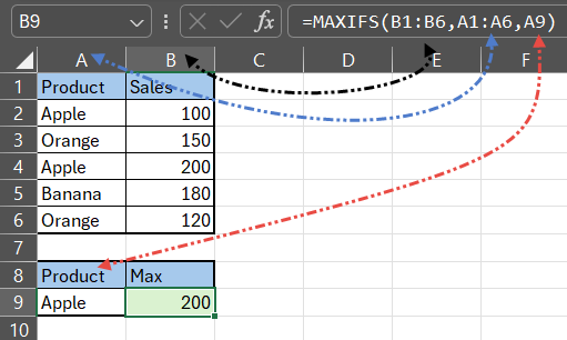
Suppose we have a sales data table with product names listed in column A and corresponding sales figures listed in column B. We want to find the maximum sales figure for a specific product.
Here’s our sales data table:

=MAXIFS(B1:B6,A1:A6,A9)This formula returns the highest sales figure among cells in column B where the corresponding product in column A is “Apple.”