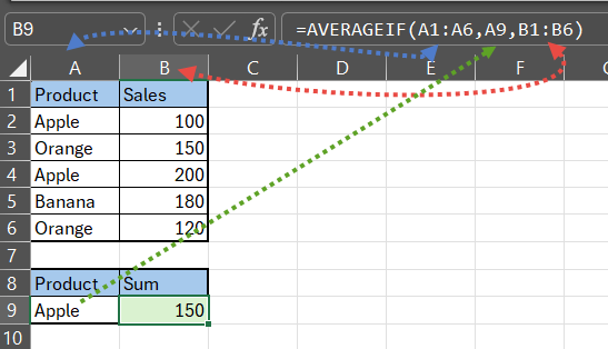
Understanding Conditional Averages:
Conditional averages in Excel involves calculating the average of values in a range that meet certain criteria or conditions. Instead of averaging all values indiscriminately, you can specify conditions that determine which values should be included in the average. This allows you to perform targeted calculations based on specific requirements or filters, resulting in more accurate and relevant results.
Conditional Average:
Excel offers several functions for performing conditional averaging, each suited to different scenarios and preferences. Let’s explore some of the most common methods:
AVERAGEIF Function:
The AVERAGEIF function calculates the average of values in a range that meet a single criterion. It takes three arguments: range, criteria, and [average_range].
range: This is the range of cells that you want to evaluate against the criteria. It can be a single row, single column, or a range of cells containing the data you want to average.criteria: This is the condition or criteria that you want to apply to the range. It can be expressed as a number, text, logical expression, or cell reference.[average_range]: (Optional) This argument specifies the actual cells to average if they meet the criteria. If omitted, Excel will average the cells in the range argument.
Here’s how you would interpret each part of the syntax:
range: The range of cells to be evaluated. For example, if you want to average values in column A based on a condition, you would specify the range asA1:A10(assuming your data is in cells A1 through A10).criteria: The condition that must be met. This can be expressed as a number, text, logical expression, or cell reference. For example, if you want to average values that are greater than 100, your criteria might be">100".[average_range]: The range of cells to be averaged. This argument is optional. If omitted, Excel will average the cells in the range argument. However, if you want to average values in a different range than the range being evaluated, you can specify the average range here. For example, if you want to average values in column B based on the condition applied to column A, you would specify the average range asB1:B10.
Putting it all together, here’s an example of how you would use the AVERAGEIF function in Excel:
=AVERAGEIF(A1:A10, ">100", B1:B10)This formula would average the values in cells B1 through B10 where the corresponding value in cells A1 through A10 is greater than 100.
The criteria values that can be used are quite flexible and can include various types of values. Here are the possible criteria values that you can use:
- Numbers: You can use numerical values directly in your criteria. For example:
">100","<50","=75", etc. - Text: You can use text values as criteria. For example:
"Apple","Banana","Completed", etc. - Logical Operators: You can use logical operators to compare values. For example:
">","<",">=","<=","=", etc. - Wildcards: Excel supports wildcards to represent one or more characters in a text string.
*(asterisk) represents any sequence of characters.?(question mark) represents any single character.
- Cell References: You can refer to the value in another cell as your criteria. For example:
A1,B2, etc. - Formulas: You can use formulas as criteria. This allows for more complex conditions based on the data in your worksheet.
- Numeric or Text Constants: You can use constants directly in your criteria. For example:
500,="Pending", etc. - Functions: Certain functions can also be used within criteria. For example, you can use functions like
LEN,LEFT,RIGHT, etc., to create dynamic criteria.
Example
Let’s say we have a sales data table with product names listed in column A and sales figures listed in column B. We want to calculate the average sales for a specific product.
Here’s our sales data table:

To calculate the average sales for “Apple,” we can use the AVERAGEIF function:
=AVERAGEIF(A1:A6, "Apple", B1:B6)This formula averages the sales figures in column B where the corresponding product in column A is “Apple.”